Capital Asset Pricing Model (CAPM)

The capital asset pricing model is an ideal interpretation of how financial markets price their securities in the market, thereby determining the expected returns on capital investments.

This model provides a theory for quantifying risk and translating it into estimates for the expected return on equity.

The capital asset pricing model is a mathematical model that explains the relationship between systematic risk and expected return for assets, especially stocks.

It is a frequently applied model in finance for pricing risky securities and calculating projected ROI based on risk and cost of capital.

What is Capital Asset Pricing Model (CAPM)?

A model for estimating capital assets was developed to react to Markowitz's modern portfolio theory, which had significant limitations due to the requirement to calculate many standard deviations and correlations for the income rates of all stocks in a portfolio.

To overcome these limitations, William F. Sharpe and John Lintner developed the CAPM model in 1964 and 1965, respectively. 

The model used the same values as the Markowitz model, namely the expected rate of return and risk, and provided a simpler way of determining an efficient portfolio of securities.

In a portfolio environment, the model proves a positive linear relationship between the needed rate of return on securities and the associated risks.

The expected return equals the sum of risk-free returns plus the risk premium from diversification. 

The model is built on a set of basic assumptions, and it establishes that investors demand a larger return for higher, more unavoidable business risk and that market equilibrium exists.

CAPM Formula & Calculation

The formula incorporates all the possible elements to arrive at the accurate and dependable expected ROI. 

Market Risk Premium is the difference between the expected market return and the risk-free market rate. It is multiplied by the beta. Which then is summed up with a risk-free rate to arrive at the Expected ROI.

CAPM is calculated through this formula

Expected return on investment = risk-free rate + beta ( market risk premium )

ERi = Rf + βi (ERM – Rf )

• ERi = Expected Return On Investment
• Βi = Beta
• ERM – Rf = Market Risk Premium
• Rf = Risk-Free Rate

1. Expected return:

The expected return is the profit or loss an investor anticipates from an investment with known historical rates of return.

It's determined by calculating possible outcomes by the likelihood of them occurring, then combining the results.

2. Risk-free-rate:

The rate of return on a speculative investment with a fixed payment schedule that is anticipated to meet all payment commitments over a set period of time. 

Given that the risk-free rate can be attained with no risk, every other risky investment will require a greater rate of return to entice investors to hold it.

Market players frequently choose the yield to maturity on a risk-free bond issued by a government of the same currency whose default risks are so minimal that they are inconsequential to deducing the risk-free interest rate in that currency.

3. Beta: 

The beta is a measurement of the volatility of an individual asset compared to the entire market. When a little asset is added to a market portfolio, beta becomes a useful measure of its contribution to the portfolio's risk.

4. Market risk premium:

A risk premium is a measure of additional return that an individual requires to compensate for exposure to a higher level of risk. It's commonly utilized in finance and economics.

Why CAPM is Important?

The capital asset pricing model is useful in financial modeling and asset appraisal. For example, when valuing a stock, a financial analyst uses the weighted average cost of capital (WACC) to calculate future cash flows' net present value (NPV).

The expected value calculated from the capital asset pricing model is used as the cost of equity (Ke) in the WACC computation. Finally, the stock's fair value is calculated by dividing the company's worth by the number of outstanding shares.

The current price of fair value is used to make an investment choice. It's a purchase if the price is less than the fair value. It's a sale if the cost exceeds the fair market value.

Example on CAPM: Let's calculate the expected return on a stock using the capital asset pricing model:

• Stock A is on the TSX exchange, and its operations are based in Canada.
• The current yield on a 5-year treasury is 3%
• The average annual return for stock A is 5.5%
• Beta is 1.15

Now:

Expected return on investment = risk-free rate + beta ( market risk premium )

Expected return on investment =  3% + 1.15 ( 5.5% )

Expected return on investment =  9.325%

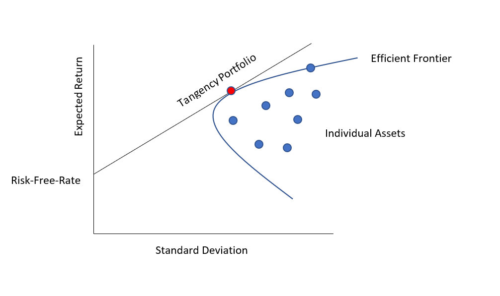
The Efficient Frontier

The CAPM is designed to assist investors in controlling risk by allowing them to build a portfolio using it. For example, as seen in the graph below, the frontier effect would exist if an investor could utilize it to optimize a portfolio's return relative to risk.

A combination of assets, for example, a portfolio, is said to be "efficient" if it has the highest expected return possible for that risk level. 

Here you can plot the possible combinations of risky assets in the risk-expected-return space. A collection of all these likely portfolios defines an area of that space.

If you don't have the opportunity to hold risk-free assets, this region is your chance set. This range's positively sloping upper bound is part of the hyperbola and is called the "efficient limit."

If risk-free assets are also available, opportunities will be greater. Its upper limit, the efficient frontier, will move out of the vertical axis at the value of risk-free asset returns, a set of risk-free asset opportunities.

All portfolios on the upper right linear boundary of the tangent portfolio are produced by risk-free borrowing. In contrast, all portfolios between risk-free and tangent portfolios are composed of risk-free and tangent portfolios.

Increase your rate and invest your earnings in your tangent portfolio.

Efficient Frontier Graph

Suppose a combination of assets, or a portfolio, has the best possible expected level of return for its level of risk (which is represented by the standard deviation of the portfolio's return). In that case, it is said to be "efficient."

In current portfolio theory, a portfolio of investments that fills the "efficient" portions of the risk-return spectrum is known as the efficient frontier (or portfolio frontier).

Formally speaking, it is the group of portfolios that meet the requirement that no other portfolios exist with higher expected returns but with the same standard deviation of return (i.e., the risk).

Although the Capital Market Line (CML) & efficient frontier are difficult to define, they demonstrate a crucial notion for investors: more yield comes at the expense of increased risk.

Because it's impossible to construct a portfolio that meets the CML, investors are more likely to take too much risk in pursuing higher returns.

The efficient frontier is based on the same assumptions as the CAPM but can only be determined theoretically.

If a portfolio were to reside on the efficient frontier, it would offer the best return for the risk it entails. 

However, because future returns cannot be forecast, it is impossible to determine whether a portfolio is on the efficient frontier.

Pros & Cons of the Capital Asset Pricing Model 

The predominant criticisms of the CAPM are across the ambiguity of the records going into the formula. 

Take the threat-unfastened price, for example. Over an analyst's selected funding time horizon, the threat-unfastened price can fluctuate now and then by simply studying the yields on treasuries in an unsettled marketplace environment.

A better threat-unfastened price could grow the cost of capital while a decreased price could lessen it-both could substantially affect the final results of a CAPM calculation. Beta also can be difficult as a degree of volatility.

Beta is calculated using a regression of historical returns. However, historic inventory returns only observe a regular distribution. 

Upward and downward rate moves are relatively safe, making a few observers wonder if it's a correct degree of threat.

Even using a historic common from a chief index is imperfect as there may be no assurance that the marketplace will perform similarly.

The CAPM stays broadly used despite its reliance on a lot of assumptions. Used as a device blended with different strategies for comparing securities, it could play a critical function in supporting analysts to make calculated decisions.

Authored & Researched by Ahmed Makki | Linkedin

Reviewed & Edited by Aditya Salunke | LinkedIn

Free Resources

To continue learning and advancing your career, check out these additional helpful WSO resources:

• Asset Turnover
• Asset Turnover Ratio
• Loan Servicing
• Loan-to-Value Ratio
• Money Laundering