Gridlines in Excel

Excel might be the greatest gift to the finance industry. What can it not do? And the funny thing is that Microsoft never takes a break from further development. For example, the Excel community thought that IF/IFS and MAX functions worked great together, so Microsoft listened and introduced the MAXIFS function in Excel 2019. 

Microsoft does not only look at its complicated formulas and functions when seeking improvement. The company also ensures that it innovates and improves basic features that offer improved usability and appreciation from the application's consumer base. 

Another tool that has always fascinated us is the horizontal and vertical lines spread across the entire spreadsheet, which can work wonders when working on complex financial models or with large data sheets.

These gray-colored lines ensure that you do not need to use additional tables or borders in spreadsheets to organize your data.

But what exactly are those lines called? Can we remove those lines from our spreadsheets if needed? Is it possible to show them in just specific areas? In this article, we will learn about Gridlines in Excel.

Gridlines - What are they?

These are the gray-colored horizontal and vertical lines that separate a spreadsheet's cells, rows, and columns. If it were not for these intersecting lines, it would have been difficult to differentiate between the data in two adjacent cells.

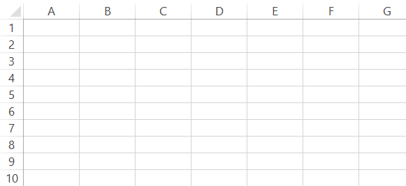
When you open the spreadsheets, the lines are visible by default. This concept is simple - Excel wants you to have organized rather than disoriented data. Unfortunately, many confuse these lines with borders, but both are entirely different things. 

These help you to work efficiently on Excel spreadsheets while using borders can add emphasis to important cells. If someone opens Excel, they will understand that the data enclosed in the frame is essential.

These grid lines can be customized with the ability to change their color, their thickness, and the pattern of the lines per the users' requirements. 

Usually, when you print an Excel file, these are ignored by default. However, you can set up a printing option in such a way that Excel prints those lines on paper.

How to remove them?

You can remove the intersecting lines from the spreadsheets in two ways. But, again, the question that might arise is why even remove the lines when it makes working on Excel easier. 

To begin with, it can make your spreadsheets more clean and tidy. Sometimes, you do not need the lines as a visual guide to align different texts and images. For example, most analysts prefer hiding these while working on various financial models. 

1. Method #1: Hiding them from the View tab

These can be turned on or off primarily by using the associated function in the ribbons bar. This is the easiest method you can follow to hide the intersecting lines in Excel. The instructions that you need to follow are:

• First, click on the 'View' tab at the top of the Excel spreadsheets.
• Next, navigate the mouse pointer to the 'Show' section and untick the checkbox for Gridlines.

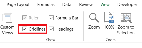
• And that's it! You will notice that all the horizontal and vertical lines have disappeared from the spreadsheets immediately.

• If you need to make the lines visible again, follow the same procedure and tick the box for 'Gridlines.' 
• Alternatively, you can use the keyboard shortcut Alt + W + VG to hide or unhide those intersecting lines in Excel.

2. Method #2: Hiding them from Options

There is another way you can hide the intersecting lines. This method lets you change the color of the lines from the traditional 'light gray' to any color you prefer. To hide the lines:

• Click on the File tab, navigate until the end to find the Options, and click on it. This will open up the dialog box as:

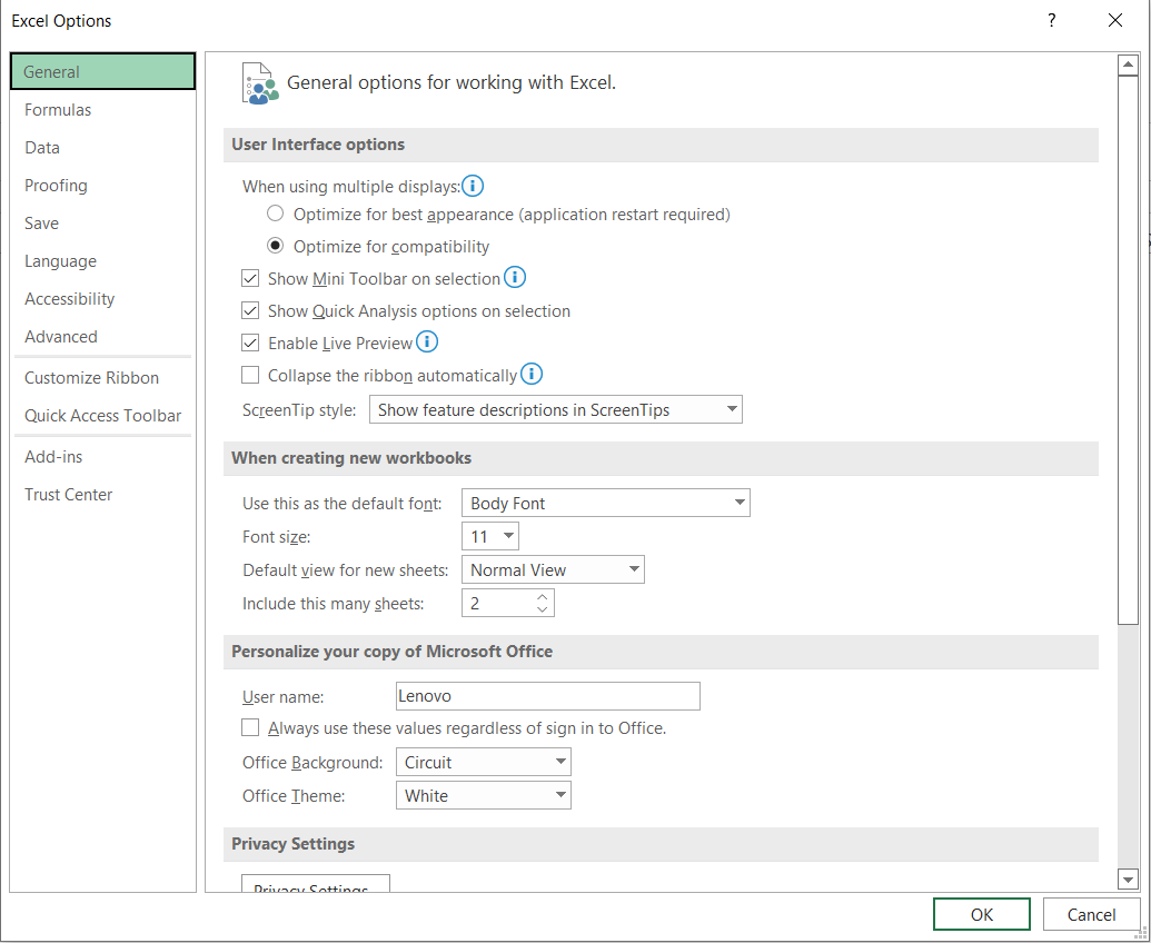
• You need to click on the 'Advanced' option on the left side and scroll down to find the section for 'Display options for this Worksheet.'

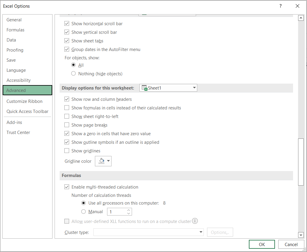
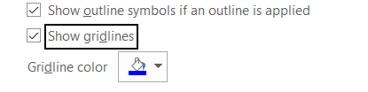
• If the lines are not visible, you need to tick the checkbox for 'Show gridlines.' But wait! That's not all, don't you like the color for the horizontal and vertical lines? 
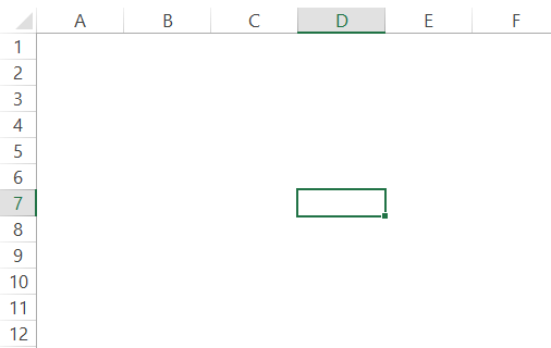
• You will find an option to change the Gridline color as well. We have changed the color to dark blue. Once done, click on the OK.

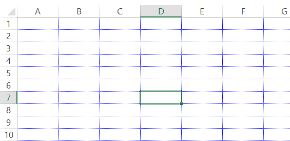
• You will find the changes in the spreadsheets as illustrated below:

Removing them from specific parts of spreadsheets

Sometimes you might need to remove the intersecting lines on a particular range of cells. Using the same technique as the above, you select the range of cells and use the keyboard shortcut Alt + W + VG to remove them. But this approach does not work.

Your logic behind hiding the lines was correct, but the method you followed does not work in Excel for a specific section of cells. So what else can you do?

Well, there are two different methods that you can follow to overcome this problem.

1. Method #1: Changing the background color

First, we will explore the 'Fill color' method to hide a specific part of lines within cells. 

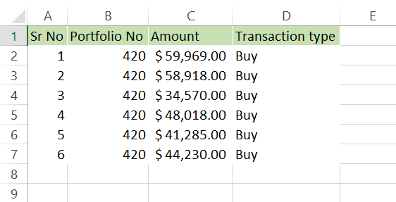
• Select the range of cells you want to remove the horizontal and vertical lines.
• Next, click on the 'Fill color' tool and select the white color. The white color will be in the first position in the color palette.

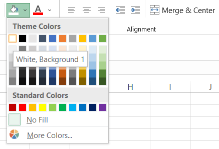
• After you have selected the color, the intersecting lines around the selected range of cells will automatically disappear.

• Since now you have selected the white color for the palette, if you need to hide the lines for other cells, select the range of cells and press the keyboard shortcut of Alt + H + H followed by the Esc key and finally press Spacebar.

2. Method #2: By changing the border's color

Another method that allows you to hide the lines around the cell is changing the border color. Since you were presented with the process behind the first method, you already know what we will do next.

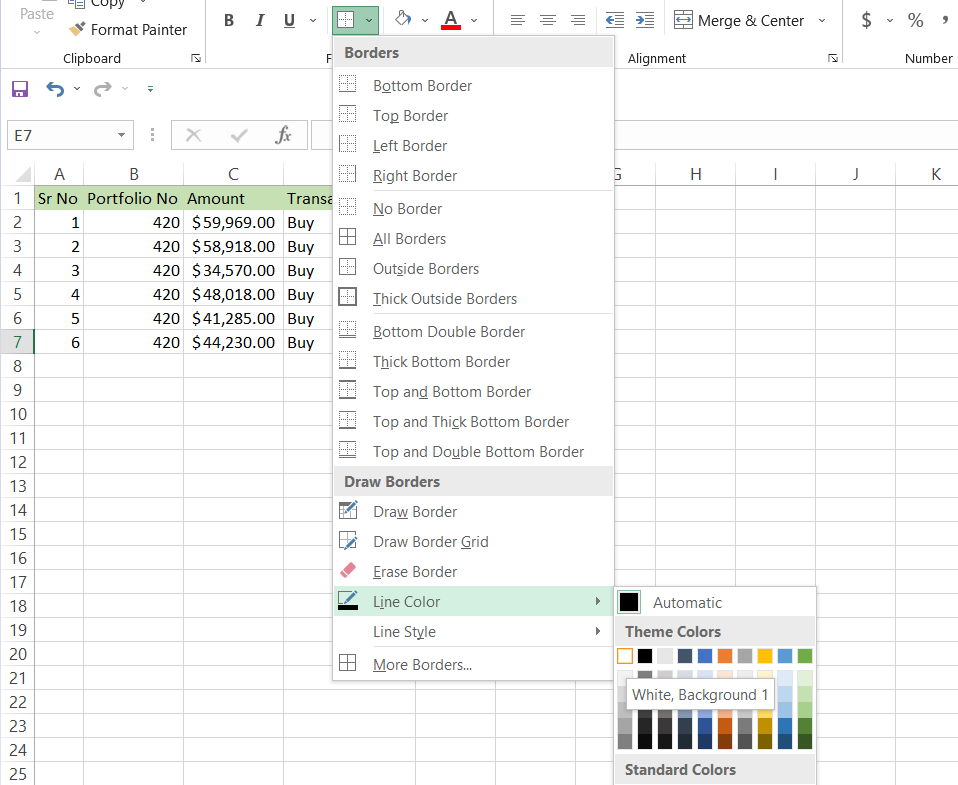
• Click on Borders that you will find in the Home tab, navigate to the 'Line Color and select the white color.

• Now, select the range of cells for which you want to hide the horizontal and vertical cells adjoining two cells.
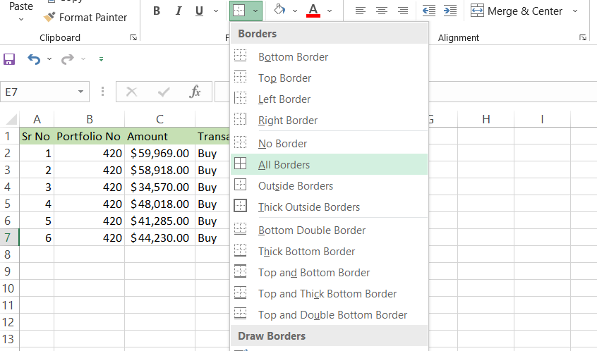
• Again, click on borders and select 'All Borders.' Why 'All Borders' though? The logic is simple; you want to hide the lines from all the sides of a cell. Of course, you may individually hide the lines, but that's just a pain in the rear.

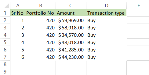
• You will get the result as illustrated below:

Removing them from multiple spreadsheets

If you press the keyboard shortcut of Alt + W + VG, you will see that all the horizontal and vertical lines separating cells disappear in the spreadsheet. However, does it also hide the gridlines on other spreadsheets in the workbook? 

Not really! There is a one-step process that you must follow to remove lines from all the spreadsheets altogether.

• Right-click on the sheet tab and select the option for 'Select All Sheets 

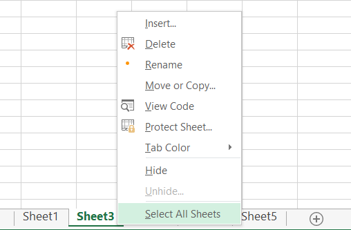
• Now you can remove the gridlines by using the keyboard shortcut of Alt + W + VG. Once done, all the spreadsheets will appear blank without horizontal and vertical lines.

Printing gridlines in Excel

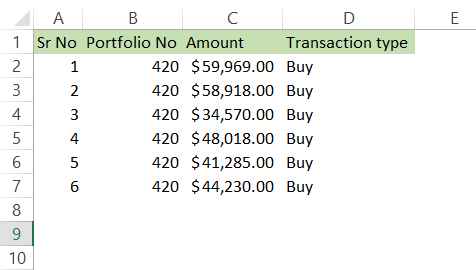
If you try to print the data from your spreadsheets, you will see that intersecting lines will not be printed. This is because excel ignores the lines since they are just for 'reference' and provides cleaner results when printed into PDFs or on paper. 

But, let's assume that sometimes you might also need to print the gridlines.

For this, you need to make a few changes in Excel.

• Click on the Page Layout tab and navigate the 'Sheet Options' section.
• For gridlines, tick the checkbox for 'Print.'

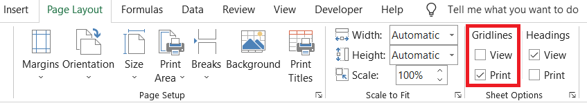
• Once you have made the changes, you should be able to print the lines along with the data from the spreadsheets.

Benefits & Drawbacks

Just as with any other application or feature, having them in the spreadsheet has its benefits and drawbacks.

Benefits

Some of the benefits of these lines in the spreadsheet are:

• With a simple keyboard shortcut of Alt + W + VG, you can hide/unhide the lines that make a great tool to have organized data.
• The intersecting lines can add equality and a better balance between two adjacent cells, making them visually appealing to the user.
• They can act as a reference for the design process for dashboards.
• Using these lines, you can divide the cells into equal proportions and have better data alignment.

Drawbacks

The drawbacks of having them in the spreadsheet are:

• 'Sometimes' these intersecting lines can hinder your creativity. For example, if you have these reference lines, all you would think is how I can fit this dashboard component in just six cells.
• Without these lines, you can set your cell size and the proportion between two adjacent cells and make changes that make the financial models much better for visually understanding.

Researched and Authored by Akash Bagul | LinkedIn

Edited by Colt DiGiovanni | LinkedIn

Free Resources

To continue learning and advancing your career, check out these additional helpful WSO resources:

• Autosum
• Developer Tab
• Excel Solver
• Excel Shortcuts
• VLOOKUP