FORECAST Function

The FORECAST function in Excel will predict a future value based on the known data using linear regression.

You may be wondering what forecasting has got to do with Excel. Well, everything.

By predicting the future with the help of past and present data, you are analyzing the trend in the numbers. This helps to make rational decisions.

If your company is low on inventory and you need to determine how much stock would be required for the next month, you can use this function to predict a value based on the preceding months statistically.

You can predict sales, expenses, or any other financial metric through financial modeling and formula. 

This article will guide you on what functions you have available to predict future numbers and how to use the FORECAST function.

The Linear Regression Equation

Since the function works on the principle of linear regression, we must understand what exactly it is. A linear regression model demonstrates a relationship between an independent and dependent variable with a straight line.

The linear regression equation is similar to the slope formula: 

Y = a + bX

where,

• Y = dependent variable
• X = independent variable
• b = slope of the line
• a = y-intercept

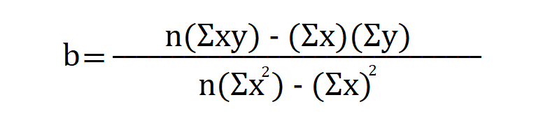
The value for a & b are further calculated using these equations:

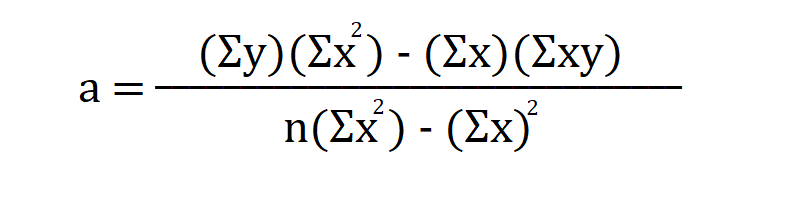
The prerequisite for linear regression is that one variable affects the other linearly.

Suppose we need to find the regression equation using the formula. We have hypothetical data for the ad revenue we at WSO generate from visitors. The data for the first five months is:

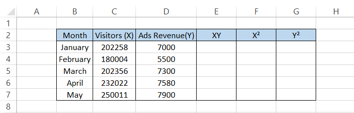
By making all the calculations in Excel, we will get the results:

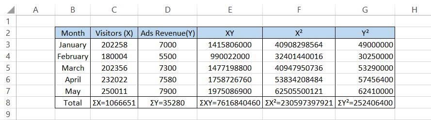
Nothing fancy, just essential addition and multiplication to derive our values in row 8. Also, we need to remember that n = 5 since our sample has five observations.

Next, we substitute those values in a & b, which will give us the values:

a = 719.41

b = 0.0297

Finally, substituting our a & b values in the regression equation, we get the result:

Y = 719.41 + 0.0297 X

And that is how we calculate the linear regression equation manually!

Different Forecasting functions

There are various forecasting functions that you can use in Excel based on which of the two methods you use:

1. Linear forecasting method-involves guessing values using linear regression.

• FORECAST - predicts a value based on existing deals with a linear trend
• FORECAST.LINEAR - introduced in the latest versions of Excel as an improved version of the earlier counterpart, FORECAST.

2. Exponential smoothing forecast-includes time series predicting for traditional data, along with seasonal or other periodic data.

• FORECAST.ETS - predicts the value for a future target date based on the exponential smoothing method
• FORECAST.ETS.CONFIDENT - predicts the confidence interval for the forecast value at a specified target date
• FORECAST.ETS.SEASONALITY - calculates the length of repetitive patterns for a given time series.
• FORECAST.ETS.STAT - calculates a statistical value based on time series forecasting.

This article will only focus on the FORECAST function that predicts a value based on linear trends. 

What is the FORECAST function in Excel

FORECAST is a statistical function that lets you predict an unknown value using the existing values and a linear trend.

It is called linear regression when you model the relationship between a dependent and independent range of values with a linear trend.

A bit difficult to understand? Let's assume the dependent value is the grade a student is in, while age is the independent value.

When the student is 11, she will be in 5th grade. When she is 12 years old, she will study in the 6th grade, and so on. So, as you can see, as age increases linearly, does the phase in which the student studies.

So, if the student's age is now 13, can you guess what grade she will be studying in? Right! The correct answer is 7th grade.

You just did a straightforward exercise of predicting based on linear trends. However, when working with a large amount of data, it becomes difficult to predict the future value of a variable in your head.

That's where the FORECAST function comes in.

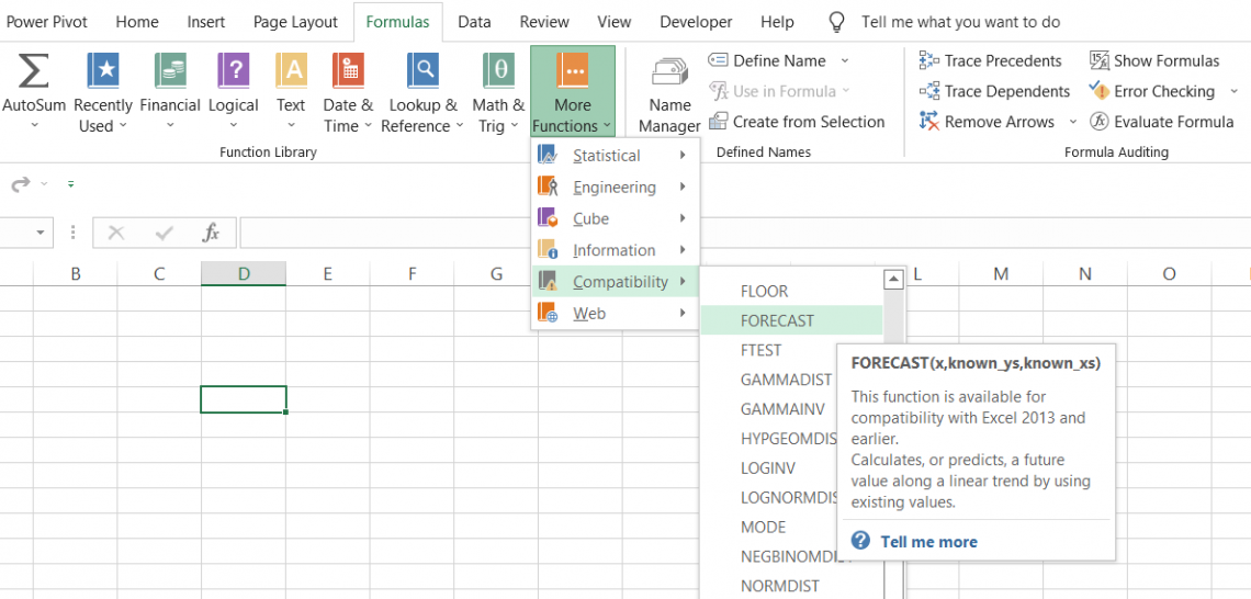
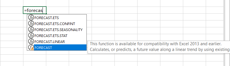
Although the function is statistical, you will find it under the Compatibility section in the More Functions tab since FORECAST replaced it.LINEAR function.

Syntax for the FORECAST function

The syntax for the FORECAST function is:

=FORECAST(x, known_ys, known_xs)

Where,

• x - (required) The numeric x-value based on which the new y-value will be predicted
• known_ys - (essential) The range of data consisting of dependent, known y values
• known_xs - (actual) The content of data composed of independent, known x values

The function was replaced with FORECAST.LINEAR in Excel 2016 and 2019. However, you can still use the position in the latest Excel versions.

If you use an older version file (2013) consisting of a FORECAST function, Excel will still display the result in your latest Excel version (backward compatibility).

Examples of the FORECAST function

This section will explore a couple of examples to understand the function better.

A) Example #1

Suppose you have the balance sheet for Apple Inc. and input the inventory values from 2018-2021. Alternatively, you can also use Yahoo Finance to get the required data, as illustrated below:

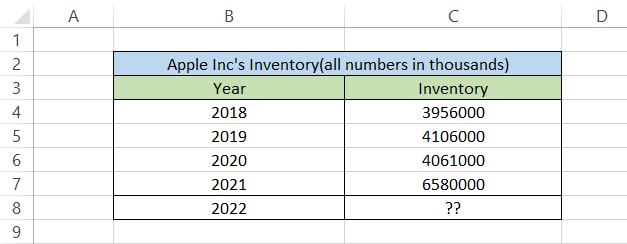
Here, our independent variable is the year, while our dependent variable is inventory.

To find the inventory requirements for the 2022 fiscal year, you will use the formula =FORECAST(B8, C4:C7, B4:B7) in cell C8 to give you the result:

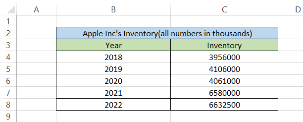
So, in 2022, Apple Inc.'s inventory requirement will be 6632500 x 103 (remember that the numbers are represented in thousands). You can also draw a graph based on your predicted value to understand the trend of the inventory requirement.

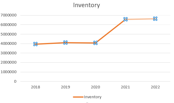
As you can see, from 2018-2020, the inventory held was stable, but then there was a sudden spike in demand for Apple Inc.'s products in 2022, with this new level expected to continue in 2022.

B) Example #2

Let's assume that we (WallStreetOasis.com) need to predict the potential website visitors for the next month and the ad revenue (not actual figures, just hypothetical) based on data from the previous months of the year.

The monthly breakdown for visitors and ad revenue is illustrated below:

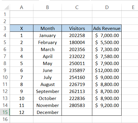
First, based on our independent value (months), we will predict the number of visitors for December.

We will use the formula =FORECAST(A15, C4:C14, A4:A14) in cell C15, giving you the monthly visitors for WSO for December as 271,856.

Next, based on our visitor count as the independent variable, we will use the formula =FORECAST(C15, D4:D14, C4:C14) in cell D15 to determine ad revenue, as illustrated below:

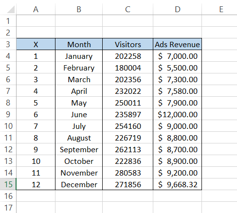
So, for December, WallStreetOasis can expect 271,856 visitors on the website and ad revenue totaling $9,668.32.

FORECAST vs FORECAST.LINEAR

You might have noticed a small yellow triangle with an exclamation mark when you use the FORECAST function. This means that the function was replaced with an equivalent process, which is FORECAST.LINEAR function.

Both functions predict a value based on the existing data, have a similar syntax and will give the same result.

The function still exists in newer Excel versions to avoid compatibility issues with older Excel versions (2013 and below).

Your client might use Excel 2013 or a prior version, and if they send a file that does not support similar functions in Excel 365, then it would be a problem.

So, Microsoft advises you to use FORECAST.LINEAR function to avoid compatibility issues, but there is nothing wrong with using either process.

The syntax for the FORECAST.LINEAR function is

=FORECAST.LINEAR(x, known_ys, known_xs)

where,

• x - (required) The numeric x-value based on which the new y-value will be predicted
• known_ys - (essential) The range of data consisting of dependent, known y values
• known_xs - (actual) The content of data comprised of independent, known x values

Let us take an example.

We will look at an example and compare the result obtained using either function to see the similarity in both positions. For example, let's say you need to predict the sales for the fourth quarter (October, November, and December) based on previous data.

The data is illustrated below:

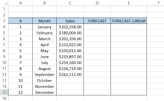
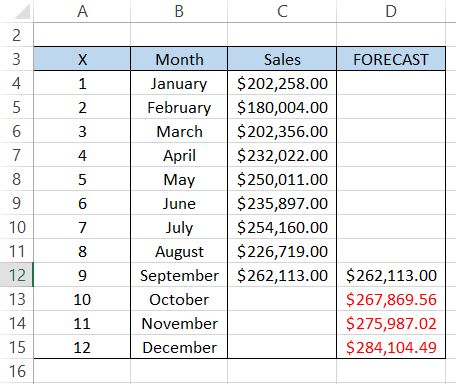
You will use the formula =FORECAST(A13,$C$4:$C$12,$A$4:$A$12) in cell D13 and drag it down to cell D15.

Similarly, in cell E13, you will use the formula =FORECAST.LINEAR(A13,$C$4:$C$12,$A$4:$A$12) to give you the result as:

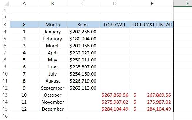
See? No difference in either result.

One more thing we understand is that we don't need to reference the initial predicted value (October sales) to find the next value (November or December).

You can drag down the formula by fixing the rows and columns, and that's it!

Next, let us prepare a graph using predicted data.

Analyzing predicted data is easier when you represent it in a graph. Though we have an entirely dedicated article on how to create graphs in excel, in this article, we will focus on preparing a line chart to portray the actual and predicted data on our graph.

Suppose that we have the sales data as illustrated below:

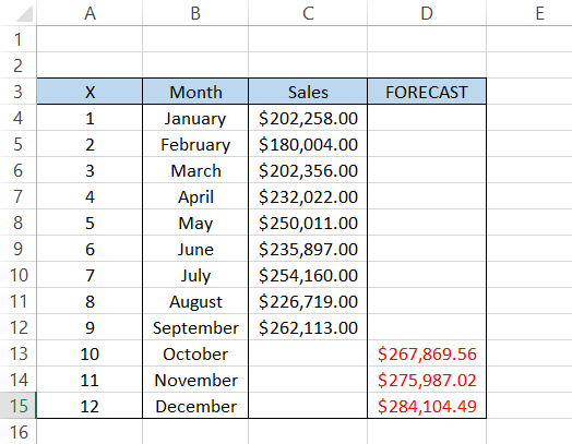
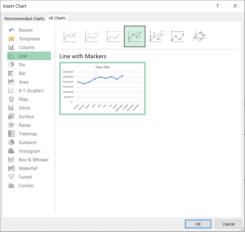
To create a line graph, follow the instructions below:

• Select the range B4:B15 and C4:C15, click on Insert > Recommended Charts > All Charts > Line, and select the 'Line with Markers' graph. Click on Ok.
• Right-click on the graph and select 'Select Data'.
• Add a new series called "Predicted" and select the range as D4:D15.
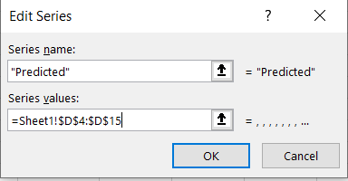
• Click on OK. The two series in the data source will look as illustrated below. Using the Edit option, you can also rename 'Series1' to 'Actual'.
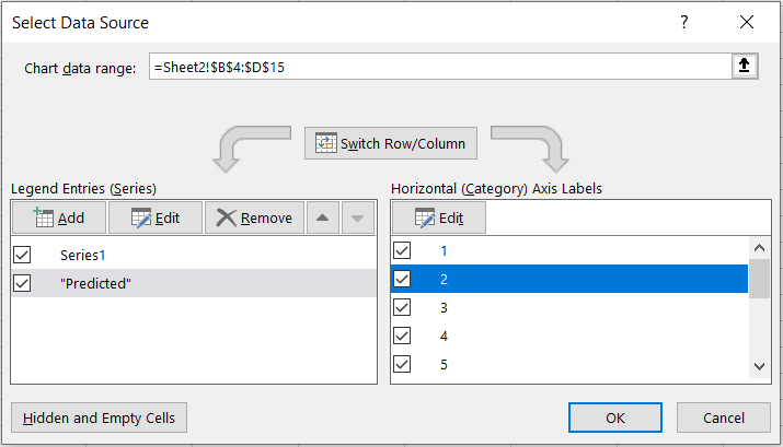
• Once the data source is added, your graph should look like this:

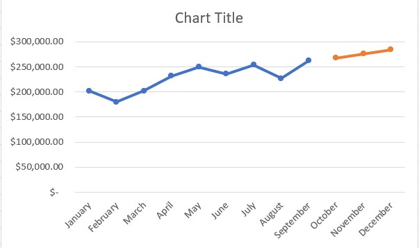
Hmm, our line graph seems to be broken. How do we deal with it? Just copy the sales in September to cell D12:

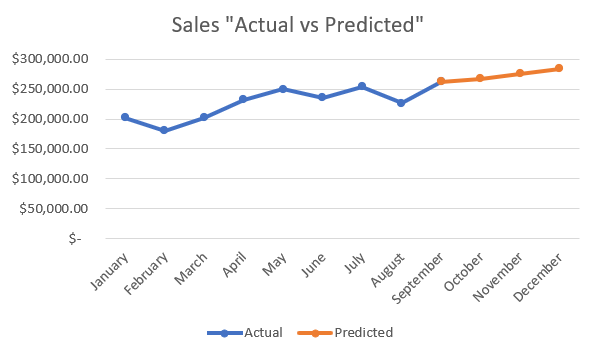
After you copy the value and customize the graph (data labels, legends, chart titles, etc.) to your liking, the final output should look something like what's illustrated below:

Important things to remember:

• If you use text for the x argument of the function, you will get a #VALUE! Error.

• If the range for known_ys and known_xs is not similar, Excel will return an #NA! error

• The variance of the known_xs should not be equal to zero, or else Excel will return a #DIV/0! Error.

Researched and Authored by Akash Bagul | Linkedin

Reviewed and edited by James Fazeli-Sinaki | LinkedIn

Free Resources

To continue learning and advancing your career, check out these additional helpful WSO resources:

• SEARCH Function
• SQRT Function
• SUBTOTAL Function
• SUM Function
• STDEVPA Function