
Excel Formulas Cheat Sheet
Helpful for Excel users in knowing the functions and how to calculate them.

Updated:
June 3, 2023Cheat sheets are helpful for anyone who wants to learn or study new equations or problems. In the case of Excel, cheat sheets are helpful for Excel users in knowing the functions and how to calculate them.

Cheat sheets help Excel users know how to use specific functions and apply them in the workbook to find the answer. They are also resourceful for Excel users in learning and creating new formulas.
Function and formula are used interchangeably, but the biggest dissimilarity between the two is that formulas are equations that the user makes. In contrast, functions are built-in calculations coded into Excel, making it easier for Excel users to calculate new formulas.
Functions are already programmed into the Excel code while the user makes formulas. For instance, =TODAY() is a function embedded into Excel that returns today's date. =TODAY()+10 is a formula as we add 10 days to today's date.
The article will give examples of how to calculate different functions and other examples of how to calculate new formulas derived from those functions.
Excel Formulas Cheat Sheet: SUM
SUM is the total amount of numeric values that are added together. This function is helpful for users who want to find the total quantity from a specified reference. For example, it can be resourceful in determining the total cost of items or the total amount of money owed.
The syntax for this function is
=SUM(number1, [number2])
where
- number1 = beginning value
- number2 = ending value. This feature is optional, but it's recommended to use it to find the sum of all the numbers we want to add.
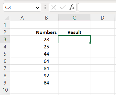
This is a very easy function to use, as all we have to do is add all the integers together. For example, suppose seven numbers are listed (28, 25, 44, 64, 84, 92, 64) in cells B3 through B9.
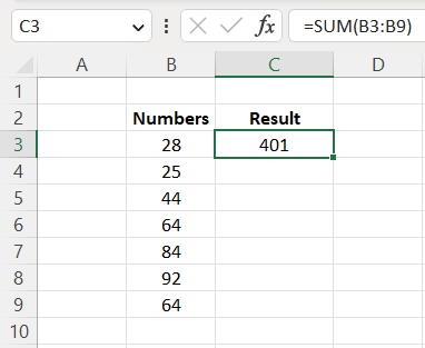
To find the total amount of those seven numbers, use the sum syntax above and input B3:B9 in the parentheses. Once done, the answer will be 401.
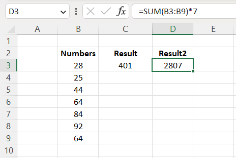
Now we know how the sum function works. Suppose we want to find the answer if multiplying it by 7. Apply those same steps to find the answer, multiply that answer by 7, and get 2,807 as the answer, as shown below.
Excel Formulas Cheat Sheet: MIN
The MIN function in Excel calculates the minimum or the smallest number from the specified sequence. It is helpful for financial analysts to calculate debt and depreciation schedules.
The syntax for MIN is
=MIN(number1, [number2])
where
- number1 = the first number selected
- number2 = the last number selected
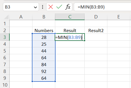
MIN is very easy to use, as all we do here is select which cells we want to be referenced, and it will return the lowest numeric value from that bunch.
Again, we have seven numbers listed (28, 25, 44, 64, 84, 92, 64), and we want to find the smallest number between those listed numeric values.
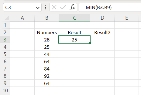
Once we've input those references in the formula, we should get an answer of 25, as that is the smallest integer listed.
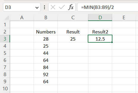
Then, we want to find our new answer if we divide that number by 3. Then, by applying the same steps we did to solve the MIN, we add "/2" at the end of the function to find the divided number and get 12.5 as our answer.
Excel Formulas Cheat Sheet: MAX
Max is an Excel operational tool that returns the largest integer within a given list of arguments. It is responsible for giving back the highest value within a specified range of cells. For example, it is useful in calculating the highest score, grade, fastest time, highest revenue amount, etc.
The syntax for MAX is
=MAX(number1, [number2])
where
- number1 = our first integer from the range
- number2 = the last integer from the range
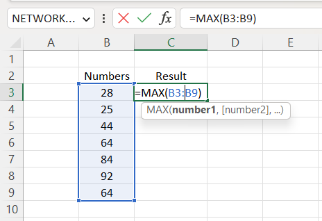
Like last time, we have seven integers being given to us. We want to determine the largest numeric value within the given range.
We want to apply that syntax by using cells B3:B9 as our reference in the parentheses.
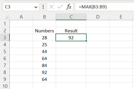
Now that we've imputed our arguments into the syntax, we should get 92 as our answer, as that is the biggest number within that range.
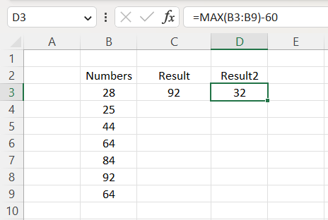
Now, suppose we wanted to know what our answer would be if we were to subtract 60 from our equation. Insert the same methods used to calculate the max and subtract it by 60; we get 32 as the answer.
Excel Formulas Cheat Sheet: Measuring Central Tendencies
We will walk through the three central tendencies in this section. The three central tendencies are Average, Median, and Mode. We will understand the three functions and show how they operate. Let's start with the Average function.

The Average function in Excel returns the arithmetic mean from a specified range of cells. It multiplies the numeric values and then divides the multiplied value by the number of cells that are being specified.
The syntax for Average is:
=AVERAGE(number1, [number2])
where
- number1 = beginning reference
- number2 = last point of reference
AVERAGE is extremely easy to use as all we have to do is insert the selected cells in the syntax, and it returns the average or the arithmetic mean from those numbers.
Like the last example, we have seven numbers (28, 25, 44, 64, 84, 92, 64) in cells B3:B9. We want to figure out what is the average between those seven numbers.
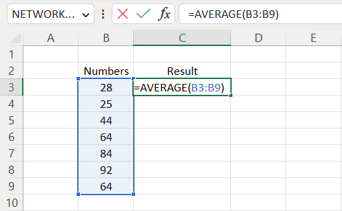
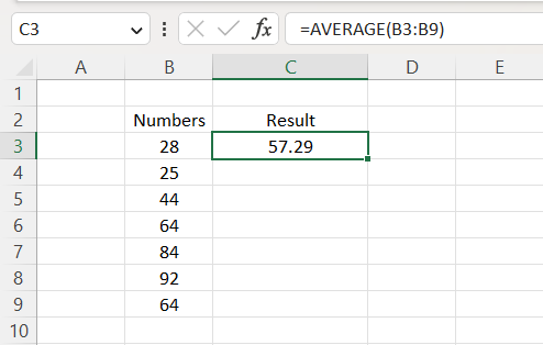
Using the average syntax, we put cells B3:B9 in the parentheses and get approximately 57.29 as our answer.
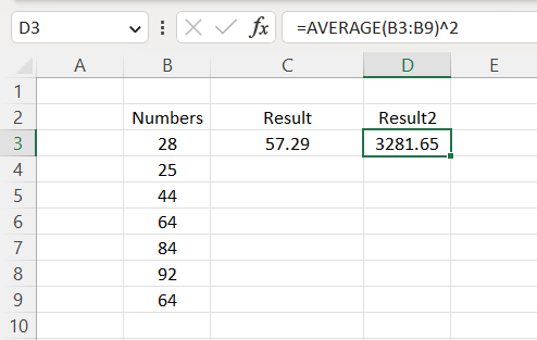
Next, we want to find out the answer if we square it. Use the same steps to calculate the average and "^2" at the tail end of the formula to find the squared integer, and we get 3,281.65 as the answer.
Now that we know what the Average function does and how its operations work, let's look at the median.
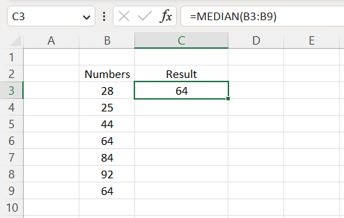
The MEDIAN is an Excel function that returns the median or the middle number from a specified set of integers. It is useful for financial analysts to determine the median of certain figures, whether it'd be median sales, median expenses, and so on.
The formula for MEDIAN is
=MEDIAN(number1, [number2])
where
- number1 = our start point.
- number2 = our endpoint.
Once again, it's not a complicated function to use as all that is required is to input the cells chosen to reference, and it should give the median number in return.
We want to determine the middle number between those integers using the same seven numbers as the previous times.
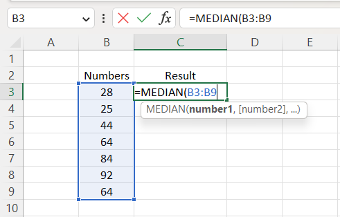
Once we have imputed those numeric values into the syntax, we got 64 as our median.
Next, we want to determine our new answer if we added 560 to 64. To find our new answer, we will have to repeat the same steps to find the minimum integer and 64 at the end of the formula, giving us 624 in return.
We seem to have a good understanding of how the median works. Finally, look at the Mode function and see how it works.
Mode is a function in Excel that returns the numeric value that occurs most often within a specific range.
It is most useful for financial analysts in determining the mode from a dataset. They can be used to determine how frequently customers buy certain products and are a very valuable marketing tool.
The syntax for MODE is
=MODE(number1, [number2])
where
- number1 = the integer we start with
- number2 = the final integer that's represented
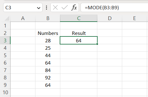
Mode is very simple to calculate. When we input the referenced cells into the syntax, the function returns the most frequent integer in that range.
We want to find the most frequently used integer within the array using the same seven numbers as before.
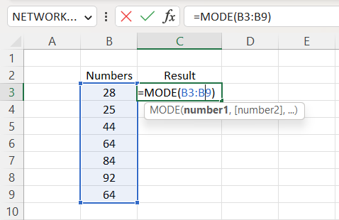
Once we've selected B3:B9 in our array, we got 64 as the answer because 64 is the only integer represented more than once.
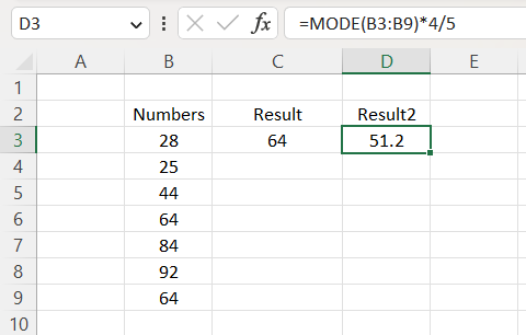
Next, suppose we want to determine our answer if we take the calculated mode and multiply it by ⅘. Using the same methods we used to calculate the mode, we would have to put "*⅘" at the end of the equation, and our answer will be 51.2.
Excel Formulas Cheat Sheet: NPV
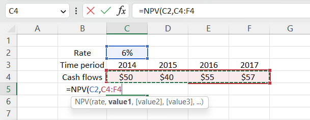
NPV is a feature in Excel that calculates the net present value of a cash flow with the discounted rate. This tool is used by financial analysts when they want to determine the values of investments.

The syntax for NPV is
=NPV(discount rate, cash values)
where
- discount rate = the rate of interest
- cash values = the cell range being represented. Cash values are labeled as value1, value2, and value3. Value1 is required, while the other values are optional.
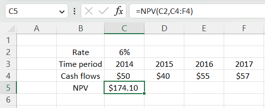
Let's say a company has compiled its cash flows for four years (2014-2017) with a discounted rate of 6%. We want to determine what the net present value is for that company. First, we would put our rate (6%) in parentheses and select cells C4:F4 for our cash value.
Once we've inputted those references in the array, we hit the enter key and return $174.10 as our net present value.
Key Takeaways
- Cheat sheets are incredibly useful for Excel users in finding new solutions.
- They are helpful for Excel users in learning how to create new formulas.
- They can be used to remember how certain functions work and operate.
- Functions are already built-in for the user, while formulas are new equations that Excel users use to figure out.

Everything You Need To Master Excel Modeling
To Help You Thrive in the Most Prestigious Jobs on Wall Street.

or Want to Sign up with your social account?