COLUMN Function in Excel

The COLUMN function is categorized as a reference/lookup function and returns the column number for a given cell reference. For example, If you use the formula =COLUMN(B3), it will return the value as 2 since B is the second column in the spreadsheet.

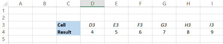
Similarly, you will get the corresponding column numbers for each cell referenced in the formula if you drag the formula horizontally.

Syntax for the Column function

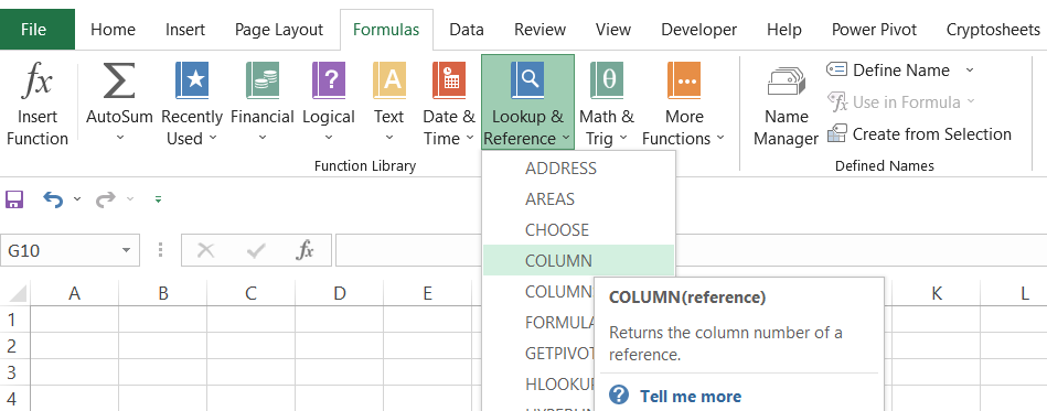
The syntax for the COLUMN function is:

=COLUMN(reference)

where,

• reference = cell reference or the range of cells for which we want to determine the column number. This is an optional argument.

Important points to remember:

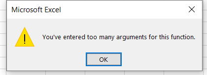
• Referencing multiple cells in a single function: When using COLUMN, you can only reference one cell at a time. So if you try to reference more than one cell, say =COLUMN(C4, D4, E4, F4), the function will not allow you to enter the parameter with an error that says:

• Referencing a range of cells in a single function: If you reference a range of cells, say D4:G4 in the function such that =COLUMN(D4:G4), the result you will get is 4 for cell D4, which is the leftmost cell in reference.

How to use the Column function

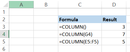
The COLUMN function is an in-built feature that is relatively easy to use. You begin with the equal sign(=), type COLUMN, and insert the cell reference to give you the column number for the referenced cell. For example, assume the three formulas in the spreadsheet provided below:

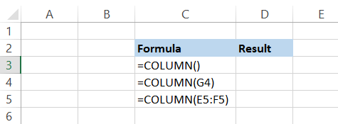
In the first formula, we have omitted the reference parameter. When we press enter, we get the result as 3, since the function assumes the reference of cell C3 in which it is used.

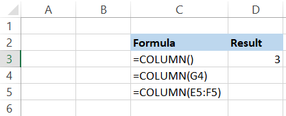
Next, we see that we have referenced cell G4 in the formula. When we press enter, the result we get is 7. The final formula consists of the range E5:F5, which returns the column number as 5 since it is the leftmost reference of our range.

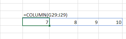
However, Excel returning our leftmost cell from the referenced range is only valid for Excel versions 2019 and below. Since Excel 365 supports dynamic array formulas, if you use the formula contained in cell C5, you will get the column numbers as an array in the form of spills in a horizontal orientation in four different cells.

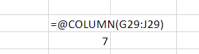
This doesn't mean that you can't get the leftmost value in Excel 365. All you need to do is add '@' after the equal sign (=), which is the implicit intersection operator (@) such that that formula becomes [email protected](G29:J29) to return the column number in the spreadsheet as:

COLUMN with the MOD function

The actual usefulness of the function is apparent when it is used along with other compatible functions such as the MOD function.

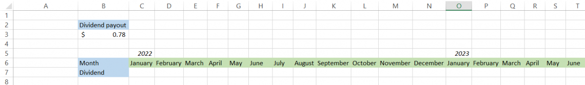
For example, assume that Company X announces a quarterly dividend payout to all its existing shareholders on 31st December 2022. The dividend that the company will pay is $0.78. This is what your spreadsheet looks like:

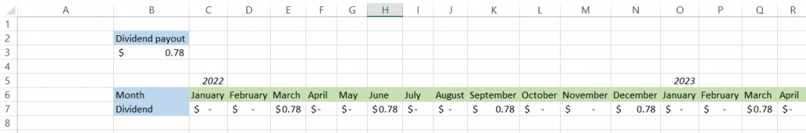
Now, it would become effortless for us to determine in which months the dividend will be paid out if a formula could be developed which would automatically assign the dividend amount at the end of every quarter. This is where COLUMN comes into the picture. The formula that you will be using is =IF(MOD(COLUMN(C7) - 2, 3) = 0, $B$3, 0)

A combination of IF, MOD, and COLUMN gives us the result in the spreadsheet as:

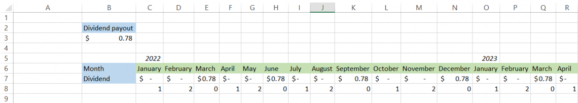
Let's break down the formula to help us understand it better. By now, you must be familiar that COLUMN returns the column number for the referenced cell, which is C7.

The function returns the column number as 3 in this example. The MOD function returns a remainder when a dividend (number A) is divided by a divisor (number B). This makes MOD a great function to return the nth column or row. By subtracting 2 from COLUMN, we return the value as 1, making it easier to highlight dividend payouts with a divisor as 3.

Whenever the column number starting from column C is returned, if it is a multiple of 3 and leaves a remainder as zero, the IF function will assign it the value of $0.78, or else it will be zero.

If the company had announced a semi-annual dividend payout in a different scenario, our divisor would have changed to 6. The formula used would become =IF(MOD(COLUMN(C7) - 2, 6) = 0, $B$3, 0) to return our result as:

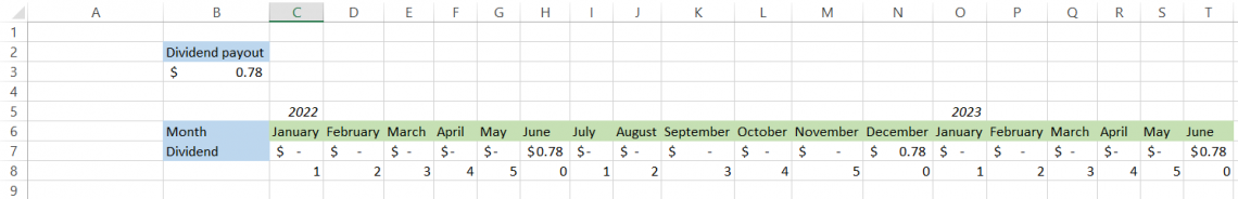
By using a conditional argument to check if the MOD + COLUMN value is equal to 0, the argument will test TRUE for the 6th, 12th, 18th value in the case of 6 as the divisor and 3rd, 6th, 9th, 12th, and so on in case of 3 as the divisor.

All the other months not falling in this criteria returned as FALSE is confirmed when the IF condition picks the dividend value from cell B3 for TRUE parameters and gives the value zero for FALSE parameters.

To learn more about the MOD function, check out our article here.

Why does proper Column referencing matter

Let's just agree that we don't always use the formulas from cell A1 itself. Sometimes you might begin from cell D3, or sometimes you might be required to return the nth column number starting from cell AD2. 

Since the columns are static, i.e., A is always equal to 1, B is always equal to 2, and so on, you need to accommodate those changes in your formula, or else it won't give you the desired result. 

We believe that it is always good to return column number as 1 while using the MOD function. The reason is quite simple - you can then use a divisor as per your convenience to return the value in the nth column.

Let us see different instances to show why it matters.

Instance 1

Assume that you purchase treasury bonds on 20th December 2022 that make semi-annual coupon payments each year for a holding period of 10 years. The formula you use to return the month in which the bond will pay the coupon is =MOD(COLUMN(B4) - 1, 6). This is what the spreadsheet should look like:

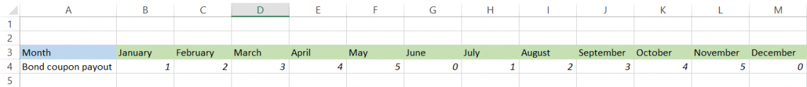
Since we have subtracted 1 from the COLUMN(B4), we get the result as 1 for the column number returned. Now, you need to make some assumptions first up to column F and then make this table displaying the coupon payments. We get this result when the same formula is used starting from column G.

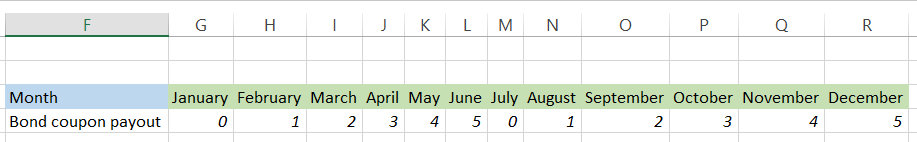
Since G is the 7th column starting from column A, subtracting 1 from it gives us column number 6, which returns the remainder as zero using the divisor.

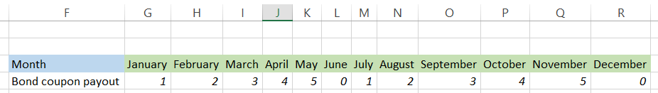
However, this is technically wrong as per our calculations about the treasury bond that makes semi-annual payments starting from the purchase date. Hence, to get the correct result, we need to amend the formula as =MOD(COLUMN(B4), 6) to start the counter again as 1.

When we drag the formula horizontally, we can expect correct coupon payments, which will be in July and December, respectively.

Instance 2

If you find it difficult to change the formula every now and then to cope with the changing columns in the spreadsheet, we have got a hack for you!

When using COLUMN, just reference it to the A1 cell and use whatever divisor you need to return the required nth column. For example, if you need to return every 5th cell, the formula will be =MOD(COLUMN(A1), 5). This way, you wouldn't have to worry about subtracting from column numbers wherever you use the formula in the spreadsheet, and it will still give you the returned column number as 1.

Instance 3

Another hack that you can use to avoid changing the formula's reference is using a double COLUMN inside the same MOD function.

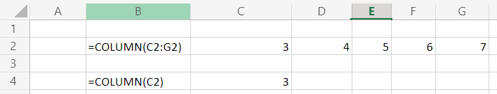
For example, COLUMN(C2:F2) - COLUMN(C2) will return the relative column number in a range. Now all you need to do is add 1 to it such that the formula becomes COLUMN(C2:F2) - COLUMN(C2) + 1, and your counter then starts from 1 for the nth term. The logic behind this is that the first COLUMN(B2:F2) will return the array as {3,4,5,6,7} while the COLUMN(C2) will only return {3}.

When the second array is subtracted from the first, you will get the array as {0,1,2,3,4}. Now, one is added, so the final array becomes {1,2,3,4,5}. You can use these formulae anywhere in the spreadsheet, and it will generate the relative column numbers in a range for that referenced range of cells.
 

SUM along with the COLUMN and MOD function

MOD and COLUMN can be combined with SUMPRODUCT to give the sum of every nth column in our dataset.

Let's assume that you have been provided with the dataset below:

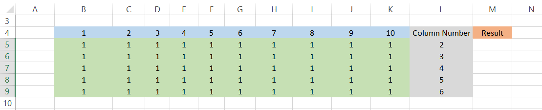
Column L represents the nth value for every column from which we will sum the value in our result.

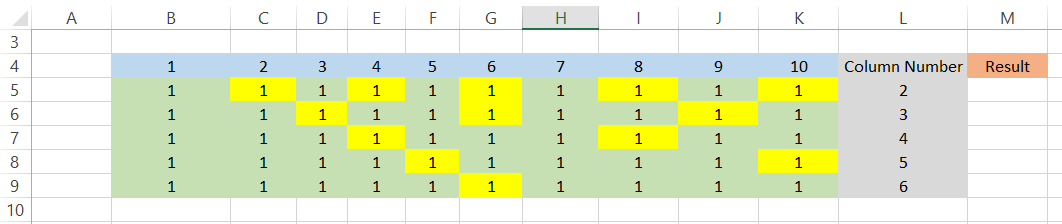
For example, suppose the value in column L is 2. In that case, it means we will go through every 2nd column from range B:K in that particular row and return the sum in column M. So for different values in column L, the corresponding values that will be pulled and whose sum will be displayed in column M are highlighted in yellow in the table below:

The formula that we will be using in cell M5 is =-SUMPRODUCT(-(MOD(COLUMN(B5:K5) - COLUMN(B5) + 1, L5) = 0), B5:K5).

Notice we have used the double negative (-) in our formula to get the result as positive. Since our MOD function gives us the array as {1,0,1,0,1,0,1,0,1,0} for row 5, the double negative changes the zero to one's and vice versa meaning the array becomes {0,1,0,1,0,1,0,1,0,1}.

Thus, all the ones from this new array indicate the nth column and return the result in cell M5. When you drag the formula down up to the cell M9, you will get the result as:

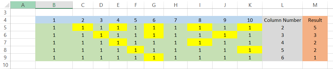
By using (COLUMN(B5:K5) - COLUMN(B5) + 1, L5), we make the formula dynamic, and it returns the same value using column functions, which are subtracted to give zero to which then one is added to return the column number as 1. 

Hence, no matter where you copy the formula, the counter for the nth column will always begin with 1.

You can compare the highlighted cells by counting the values in each row and their corresponding sum in the cells of column M to find that they perfectly match. Think of it this way, the formula creates a logic that skips the cell values until it finds a column number that is divisible by our value in column L to give the remainder as zero which is when the number is added to the final sum.

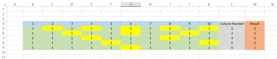
Additionally, you could tweak your formula so that if any of the values from the row, especially if your nth value is zero, the result in column M will return zero as well. All you need to do is add COUNTIF function along with the IF conditional statement in the beginning such that your formula becomes =IF(COUNTIF(B5:K5, "0"), 0, -SUMPRODUCT(-(MOD(COLUMN(B5:K5) - COLUMN(B5) + 1, L5) = 0),B5:K5)). 

If any of the highlighted values are turned to zero as in cell I5, the result in M5 will also return to zero.

Practical Example #1

Suppose that you have a certain requirement in your spreadsheet where column F should contain the value as FALSE. 

Here, you can use the combination of SUBSTITUTE and COLUMN to derive column F and then include a conditional IF statement to return the value as FALSE if it is column F and do nothing if it is another column.

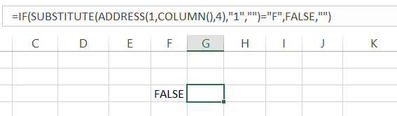
The formula that you will be using here is =IF(SUBSTITUTE(ADDRESS(1, COLUMN(), 4), "1", "") = "F", FALSE, ""). If you copy this formula in any of the cells in column F, the value you will get is FALSE. However, copy it to any other column, and the value that will return is an empty cell. After using the formula in cells F1 and G1, respectively, your spreadsheet will look like this:

If you break down the formula, the ADDRESS function basically returns the cell reference that we set up in the formula. The syntax for the ADDRESS function is:

=ADDRESS(row_num,col_num, [abs_num], [a1], [sheet])

where,

• row_num = row number that will be used in the cell address
• col_num = column number that will be used in the cell address
• abs_num = This is an optional parameter that defines whether the address type is relative or absolute
• a1 = This is an optional parameter that determines reference style i.e R1C1 or A1 style
• sheet = refers to the worksheet where the formula will be used. This is another optional parameter

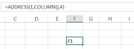
If we use just the ADDRESS function such that =ADDRESS(1, COLUMN(), 4) we get the result as F1. Since row_num is of less significant importance here (use any number as row_num, and still you will get the same final result for COLUMN), the critical parameter is the col_num which is represented by COLUMN() in our formula.

As the reference is missing inside the parenthesis, it assumes the column's value in which the function is present. Finally, the abs_num parameter as 4 means relative referencing is selected, i.e., neither rows nor columns are frozen, which you can usually do by pressing the F4 key on the keyboard.

Next, we just substitute the 1 from our result F1 using the function SUBSTITUTE to just give the value as F. Finally, the IF condition checks if the value is F and returns as FALSE or else just an empty cell.

The syntax for the SUBSTITUTE function is:

=SUBSTITUTE(text, old_text, new_text, [instance])

where,

• text = the referenced text 
• old_text = the part of the referenced text that needs to be replaced
• new_text = The text that will be used to replace the old_text
• instance = the instance to replace

More on Excel

To continue your journey towards becoming an Excel wizard, check out these additional helpful WSO resources.

• Excel keyboard shortcuts for Windows and Mac
• Advanced Excel formulas you must know
• Excel modeling best practices
• Developer tab
• INDEX MATCH formula in Excel