Autosum

AutoSum is an Excel shortcut that automatically adds all the numbers in the selected range. Since SUM is one of the most popular functions in Excel (check here top 10 popular Excel functions), Microsoft created the AutoSum function that is of special importance among Excel users.

Financial analysts spend hours on end performing complex calculations in Excel. By using shortcut keys, they can potentially save a lot of time cumulatively that they can invest somewhere else (Yes, we all love tea breaks with our colleagues more than staring at Excel Models).

In this article we will show you two ways you can use the AutoSum function to calculate the sum of the numbers in your spreadsheet.

Method 1: Keeping it simple

Most analysts prefer to use keyboard over mouse while working on spreadsheets and by extension, shortcut keys. If you are one of those Excel users, you can use the keyboard shortcut of Alt and the = keys to sum the rows or columns. 

Pressing the Alt key with the equal sign (=) key simultaneously inserts a SUM function in the cell just like manually typing the =SUM(A:A) in the cell. Finally press Enter to get the result for the AutoSum function.

And there you have it! Just a combination of two keys to use one of the most popular excel functions.

An example showing the AutoSum function in action is illustrated below:

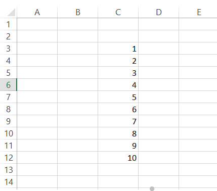
The spreadsheet shows a series of vertical and horizontal numbers for which the sum is to be calculated.

First we will see how the function works for the vertical series of numbers.

Navigate to the cell C13 using the keyboard arrow keys and press the Alt and the = key together. You will see the formula displayed in the cell as:

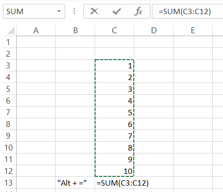
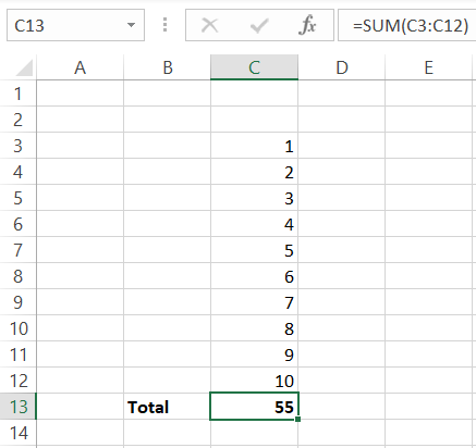
Finally press the Enter key and the function will give the result as 55.

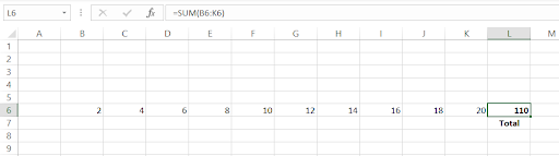
Similarly the function can be used for horizontally ranged cells containing values using the same key combination.

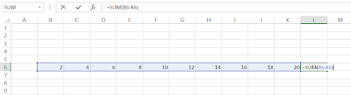
The result for the Autosum function for the selected cells is given in the cell L6.

That's it. This example shows the importance of the AutoSum function. So does this article end here? Definitely not! No two financial analysts think the same way. That's why we need to show you the alternate way to use the AutoSum function.

Method 2: Keeping it simple, but using the Excel ribbon

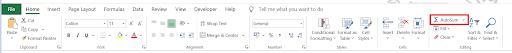
You can find the AutoSum function in two different places in the Excel ribbon. First, you can find it in the Home tab in the Editing section.

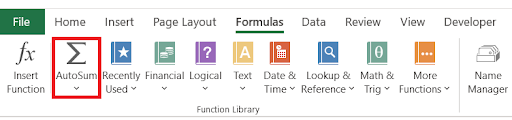
Second, you can use the AutoSum by clicking on Formulas tab and find it in the function library as below

To understand how to use the AutoSum from the Excel ribbon, consider the example below:

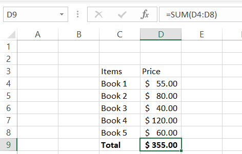
The price of the five different books is given in the spreadsheet below. 

First, select the cell D9 which will be our resultant cell for the sum. Click on the Home tab and click on the AutoSum function to display the formula in cell D9.

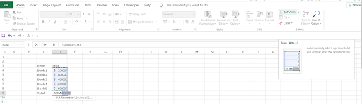
Finally, press Enter to get the result of the function. The cell will display $355.00 as the sum of all the books. Similarly you can use the keyboard shortcut of Alt + H + U + S to use the AutoSum for vertical and horizontal sums and press Enter to give the result in the desired cell.

Using AutoSum for filtered cells

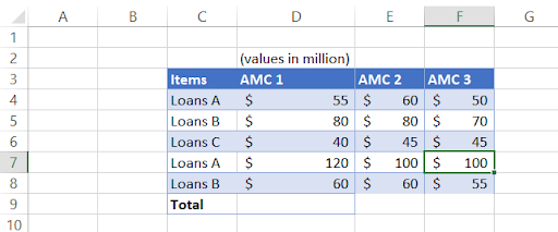
Let's assume that an asset management company has three types of loans A, B & C. You, as an analyst, need to calculate the total sum of loan A to reconcile the loans booked.

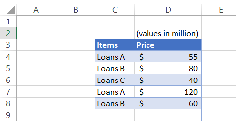
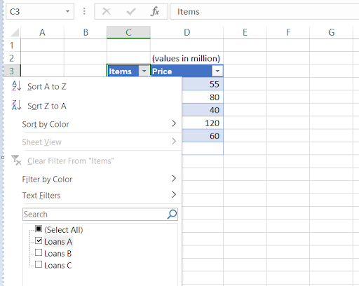
To do this, first you need to convert the data into a table using the Excel shortcut Ctrl + T or you can just use the filter to select the desired Loan, i.e., Loans A and press Enter.

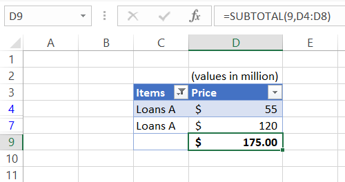
Now use the keyboard shortcut of Alt and = and it will give you the subtotal of all the Loans A in your data which is equal to $175.

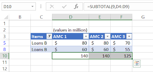
Using AutoSum on more than one cell

You can use the AutoSum function on multiple cells by simply selecting those cells and using the keyboard shortcut of Alt + = and finally pressing the Enter key.

Suppose that three different asset management companies have Loan A, B & C that need to be booked. We need to find the total amount of Loans B for all three asset management companies. You can do this by selecting the range D5:F10 and using the AutoSum function. The spreadsheet will give the result as below:

Similarly this can be done for a horizontal set of data or the combination of horizontal and vertical. 

Common issues while using the AutoSum function

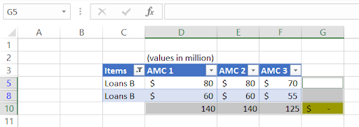
Let's see how we use the AutoSum function to find the sum for both horizontal and vertical dataset. We are calculating the total sum of loan B in different AMC's (vertical sum) as well as how much of loan B do each of the AMCs hold (horizontal sum).

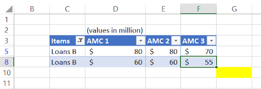
For this, we have first added the filter to column C and set the values to Loans B. Next we will be selecting the range which in this case is D5:G10.Use the keyboard shortcut of Alt and = which will lead to the following result:

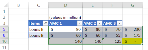
If you had done this by selecting only the range D11:G11 & G5:G11, you would get an incomplete result for either horizontal or vertical sum but not both together. 

Another common issue that you can face is when the numbers are formatted as text. In such cases, it will not include them in the calculations as Excel considers them as a text string. 

If there is a small green triangle in the top left corner of the cell in which the number exists, you will need to convert those texts to numbers by clicking on the warning sign and select the option for Convert to Number (This can be a problematic issue while working with the VLOOKUP & XLOOKUP as well!).

Autosum vs. Sum

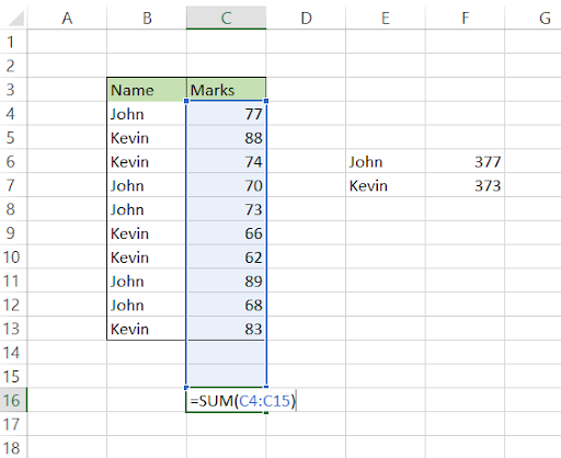
If you intend to use Autosum on the full range of cells and skip a few empty cells in the process, it will sum the result for the referenced range including the blank cells. For example, let's say you expect the marks of three more subjects to be added for your grand total. We have left three blank cells after which we have used the Autosum function in cell C16 using Alt and = sign. 

This will result in the total of 685 in cell C16. Now after a couple of days, once you receive the marks for the last three subjects, you can directly input those numbers in the empty cells which will give you the updated total in cell C16 without changing any reference for our formula.

In case more rows are added between the table, the autosum function will incorporate those cells as the reference for sum in the function.

The only difference between Autosum and Sum is that the latter will displays the result just below the range of cells either for both row and column values, as opposed to the former which takes blank cells into account. 

Autosum vs. Addition (+)

The biggest difference between using Autosum and Addition (+) is that the latter will allow you to do manual addition as the name suggests. 

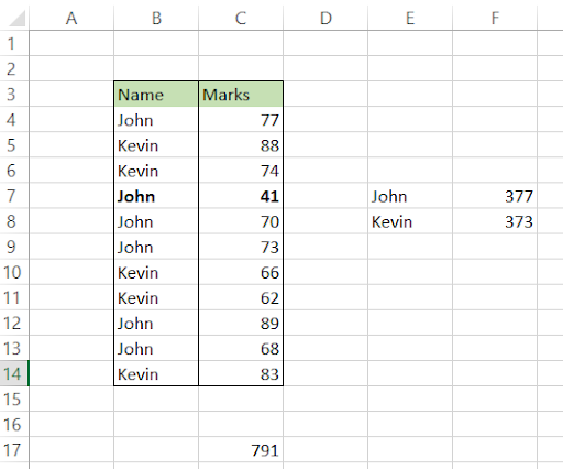
Let's understand this with the help of an example: John and Kevin make a table based on the marks they had obtained in different subjects. They want to now determine what is the total marks they obtained out of 500.

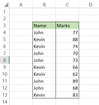
Here, they can manually add the marks for John and Kevin respectively.

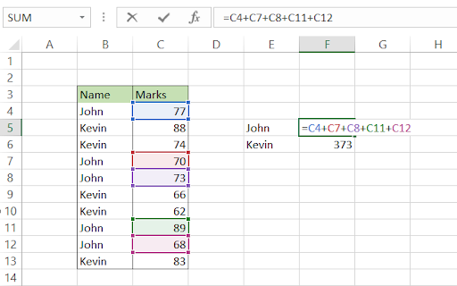
If we had used Autosum here, the result would also have incorporated the marks for Kevin as well in our result.

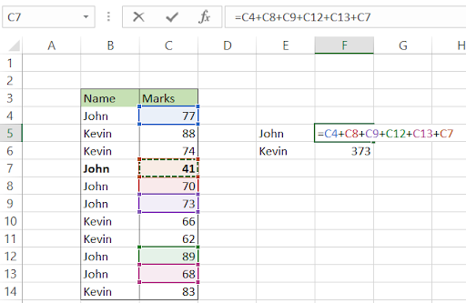
Another big difference between both the Sum methods is the addition of new values between the referenced cells. Suppose, you add a new row below cell B6 with values "John" and "41". If you check your total in cell F6, it remains the same. However, your AutoSum total for the marks obtained by both John and Kevin increases by 41 to 791 in cell C16. 

To include this new value, your formula in cell F6 becomes =C4+C8+C9+C12+C13+C7 where we have included the reference to the value as cell C7. Though using either method has its pros and cons, you can improve your work efficiency, precision and productivity by using them at different situations.

More on Excel

To continue your journey towards becoming an Excel wizard, check out these additional helpful WSO resources.

• Excel keyboard shortcuts for Windows and Mac
• Advanced Excel formulas you must know
• Best Excel courses
• Excel modeling best practices
• Add Months to Date